Are Two Separate or Independent Groups Different
When Variable Expressed by Proportions?
z Distribution
One very special member of the normal distribution family is called the standard normal distribution, or Z-distribution.
In statistics, the Z-distribution is used to help find probabilities and percentiles for regular normal distributions (X). It serves as the standard by which all other normal distributions are measured.
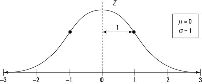
The Z-distribution is a normal distribution with mean zero and standard deviation 1; its graph is shown here. Almost all (about 99.7%) of its values lie between –3 and +3 according to the Empirical Rule. Values on the Z-distribution are called z-values, z-scores, or standard scores. A z-value represents the number of standard deviations that a particular value lies above or below the mean. For example, z = 1 on the Z-distribution represents a value that is 1 standard deviation above the mean. Similarly, z = –1 represents a value that is one standard deviation below the mean (indicated by the minus sign on the z-value). And a z-value of 0 is — you guessed it — right on the mean. All z-values are universally understood.
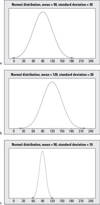
The above figure shows some examples of normal distributions. To compare and contrast the distributions shown here, you first see they are all symmetric with the signature bell shape. Examples (a) and (b) have the same standard deviation, but their means are different; the mean in Example (b) is located 30 units to the right of the mean in Example (a) because its mean is 120 compared to 90. Examples (a) and (c) have the same mean (90), but Example (a) has more variability than Example (c) due to its higher standard deviation (30 compared to 10). Because of the increased variability, most of the values in Example (a) lie between 0 and 180 (approximately), while the most of the values in Example (c) lie only between 60 and 120.
Finally, Examples (b) and (c) have different means and different standard deviations entirely; Example (b) has a higher mean which shifts the graph to the right, and Example (c) has a smaller standard deviation; its data values are the most concentrated around the mean.
Note that the mean and standard deviation are important in order to properly interpret values located on a particular normal distribution. For example, you can compare where the value 120 falls on each of the normal distributions in the above figure. In Example (a), the value 120 is one standard deviation above the mean (because the standard deviation is 30, you get 90 + 1[30] = 120). So on this first distribution, the value 120 is the upper value for the range where the middle 68% of the data are located, according to the Empirical Rule.
In Example (b), the value 120 lies directly on the mean, where the values are most concentrated. In Example (c), the value 120 is way out on the rightmost fringe, 3 standard deviations above the mean (because the standard deviation this time is 10, you get 90 + 3[10] = 120). In Example (c), values beyond 120 are very unlikely to occur because they are beyond the range where the middle 99.7% of the values should be, according to the Empirical Rule.
Now, based on the above figure and the discussion regarding where the value 120 lies on each normal distribution, you can calculate z-values. In Example (a), the value 120 is located one standard deviation above the mean, so its z-value is 1. In Example (b), the value 120 is equal to the mean, so its z-value is 0. Example (c) shows that 120 is 3 standard deviations above the mean, so its z-value is 3.
+++++++++++++++
When a study uses nominal or binary (yes/no) data, the results are generally reported as proportions or percentages.
The binomial distribution introduced in Chapter 4 can be used to determine confidence limits or to test hypotheses about the observed proportion.
Recall that the binomial distribution is appropriate when a specific number of independent trials is conducted (symbolized by n), each with the same probability of success (symbolized by the Greek letter π), and this probability can be interpreted as the proportion of people with or without the characteristic we are interested in. Applied to the data in this study, each shunt placement is considered a trial, and the probability of having an infection in the ≤1 year age group is 8/47 = 0.170.
The binomial distribution has some interesting features, and we can take advantage of these. Figure 5–4 shows the binomial distribution when the population proportion π is 0.2 and 0.4 for sample sizes of 5, 10, and 25. We see that the distribution becomes more bell-shaped as the sample size increases and as the proportion approaches 0.5. This result should not be surprising because a proportion is actually a special case of a mean in which successes equal 1 and failures equal 0, and the central limit theorem states that the sampling distribution of means for large samples resembles the normal distribution. These observations lead naturally to the idea of using the standard normal, or z, distribution as an approximation to the binomial distribution.++++++++++++++
[ In medicine we sometimes observe a single group and want to compare the proportion of subjects having a certain characteristic with some well-accepted standard or norm.]